Complex GIS in R

An in-depth look at spatial dataset analyses.

Complex GIS

So now we know how to read in, create and download different sources of Vector data and Rasters, use and combine these data to produce maps. Now lets look at using some of these skills but combining different data sources, converting between different resolutions and dimensions, converting between data types and then create summary statistics within spatial limits.

What is our Objective?

Through my work, I often have a habitat classification of an area that has a resolution and dimension of the original imagery and then we want to compare this classification to other environmental data, such as temperature, solar radiation or salinity. However, very rarely will the open access environmental data align with the habitat classification. So we will look at habitat classification of an area with a specific (maybe illogical) resolution and dimension, then we will relate these environmental data to then split the environmental data by its classification.

Input Data

First: Habitat Classification

We could create our own classification model and use the output of that but to stick to our objective we will download a classification from r package. This will come from the geodata package, where there is an example of the CORINE landcover classification of the Island São Miguel from the Azores. This has a lot of complicated groups (23 to be exact) so we will combine them into more general groupings. We can use tidyterra to do this,which mimics tidyverse methods.

library(exactextractr)
library(sf)
library(terra)
library(tidyterra)
library(tidyverse)


classification <- rast(system.file('sao_miguel/clc2018_v2020_20u1.tif',
                     package = 'exactextractr')) 

print(unique(classification$LABEL3))

                                                                                   LABEL3
1                                                                 Continuous urban fabric
2                                                              Discontinuous urban fabric
3                                                          Industrial or commercial units
4                                                                              Port areas
5                                                                                Airports
6                                                                Mineral extraction sites
7                                                                              Dump sites
8                                                                      Construction sites
9                                                                       Green urban areas
10                                                           Sport and leisure facilities
11                                                              Non-irrigated arable land
12                                                      Fruit trees and berry plantations
13                                                                               Pastures
14                                                           Complex cultivation patterns
15 Land principally occupied by agriculture, with significant areas of natural vegetation
16                                                                    Broad-leaved forest
17                                                                      Coniferous forest
18                                                                           Mixed forest
19                                                                     Natural grasslands
20                                                                    Moors and heathland
21                                                            Transitional woodland-shrub
22                                                                           Water bodies
23                                                                          Sea and ocean

Grouped_Classification<-classification%>% 
  tidyterra::mutate(LABEL3=case_when(
    LABEL3%in%c("Continuous urban fabric",
                  "Discontinuous urban fabric",
                  "Industrial or commercial units",
                  "Port areas",
                  "Airports",
                  "Mineral extraction sites",
                  "Dump sites",
                  "Construction sites",
                  "Green urban areas",
                  "Sport and leisure facilities")~"Urban",
      LABEL3%in%c("Broad-leaved forest",
                  "Coniferous forest",
                  "Mixed forest",
                  "Natural grasslands",
                  "Moors and heathland",
                  "Transitional woodland-shrub")~"Wild Vegetation",
      LABEL3%in%c("Water bodies",
                  "Sea and ocean")~"Ocean/Water Body",
      TRUE~"Farmland")
                    )

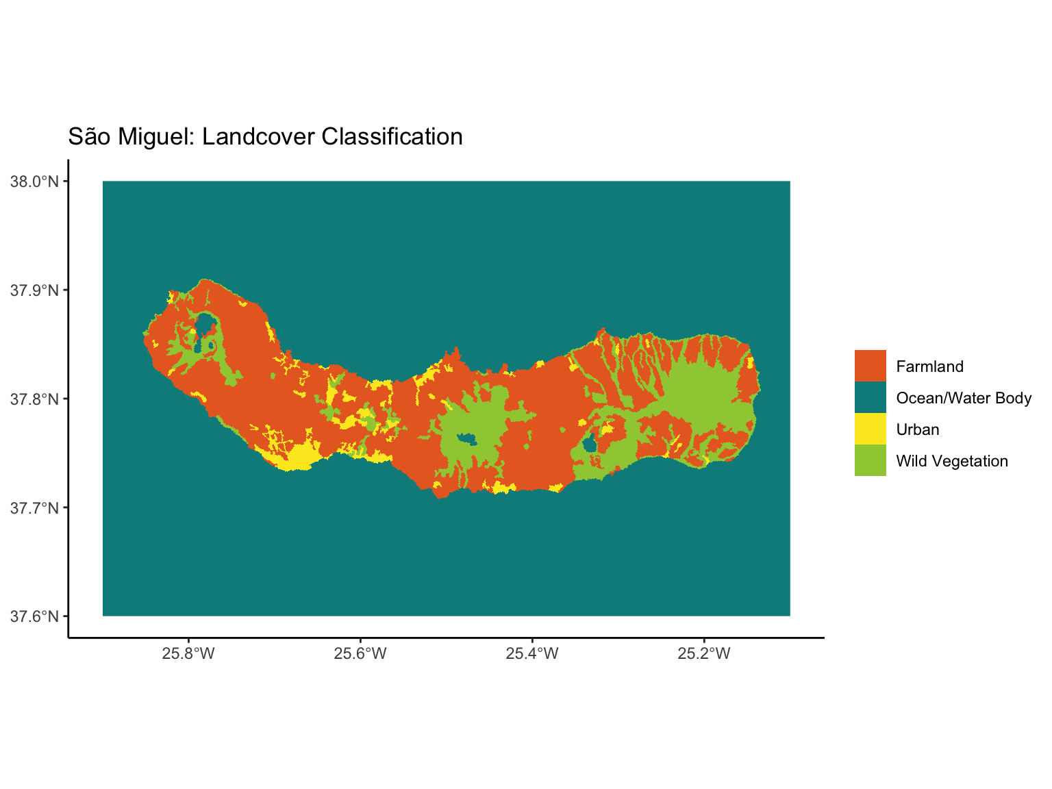
ggplot()+
  geom_spatraster(data=Grouped_Classification,
                  maxcell = 5e+7
                  )+
  labs(title="São Miguel: Landcover Classification")+
  scale_fill_manual(name="",
                    values = c("#e86a28","#008B8B", "#fde825", "#9fcb41"))+
  theme_classic()

Second: Environmental Data

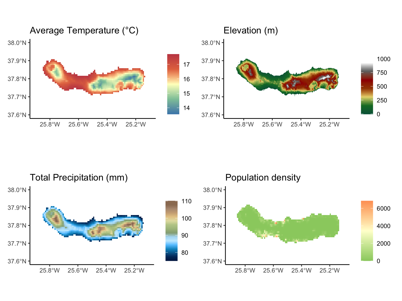
We have already previously downloaded climate data from the geodata package, we can do this again for the same extent as our Habitat data, we will download temperature, elevation, precipitation and population density. Again as before some data will be a layer for each month, so we will average across the layers.

library(geodata)
library(patchwork)

avgtemp <- worldclim_tile(var="tavg",
                          lon=-25.5,lat=37.8,
                          path=tempdir())

avgtemp_SM<-avgtemp %>% 
  crop(Grouped_Classification)%>% 
  mean()

p1<-ggplot()+
  geom_spatraster(data=avgtemp_SM)+
  labs(title="Average Temperature (°C)",fill="")+
  scale_fill_whitebox_c("muted",na.value = NA)+
  theme_classic()


Elevation_SM<-elevation_3s(lon=-25.5,lat=37.8, 
                           path=tempdir())%>% 
  crop(Grouped_Classification)

p2<-ggplot()+
  geom_spatraster(data=Elevation_SM)+
  labs(title="Elevation (m)",fill="")+
  scale_fill_hypso_c("dem_poster",na.value = NA)+
  theme_classic()

avgprec_SM <- worldclim_tile(var="prec",lon=-25.5,lat=37.8,
                             path=tempdir())%>% 
  crop(Grouped_Classification) %>% 
  mean()

p3<-ggplot()+
  geom_spatraster(data=avgprec_SM)+
  labs(title="Total Precipitation (mm)",fill="")+
  scale_fill_hypso_c("colombia",na.value = NA)+
  theme_classic()


pop_density <- rast(system.file('sao_miguel/gpw_v411_2020_density_2020.tif',
                                  package = 'exactextractr'))

p4<-ggplot()+
  geom_spatraster(data=pop_density)+
  labs(title="Population density",fill="")+
  scale_fill_whitebox_c("soft",na.value = NA)+
  theme_classic()


(p1+p2)/(p3+p4)

Comparing Reference Systems, Resolutions and Extents.

Before we combine all these data together and start assessing potential patterns we will want to make sure our data are at comparable coordinate reference systems, resolutions and extents.

crs(Grouped_Classification,describe=T)
crs(avgtemp_SM,describe=T)
crs(Elevation_SM,describe=T)
crs(avgprec_SM,describe=T)
crs(pop_density,describe=T)

res(Grouped_Classification)
res(avgtemp_SM)
res(Elevation_SM)
res(avgprec_SM)
res(pop_density)

ext(Grouped_Classification)
ext(avgtemp_SM)
ext(Elevation_SM)
ext(avgprec_SM)
ext(pop_density)

    name authority code  area             extent
1 WGS 84      EPSG 4326 World -180, 180, 90, -90
    name authority code  area             extent
1 WGS 84      EPSG 4326 World -180, 180, 90, -90
     name authority code area         extent
1 unknown      <NA> <NA> <NA> NA, NA, NA, NA
    name authority code  area             extent
1 WGS 84      EPSG 4326 World -180, 180, 90, -90
    name authority code  area             extent
1 WGS 84      EPSG 4326 World -180, 180, 90, -90
[1] 0.0002083333 0.0002083333
[1] 0.008333333 0.008333333
[1] 0.0008333333 0.0008333333
[1] 0.008333333 0.008333333
[1] 0.008333333 0.008333333
SpatExtent : -25.9, -25.100000000128, 37.600000000064, 38 (xmin, xmax, ymin, ymax)
SpatExtent : -25.9, -25.1, 37.6, 38 (xmin, xmax, ymin, ymax)
SpatExtent : -25.9, -25.1, 37.6, 38 (xmin, xmax, ymin, ymax)
SpatExtent : -25.9, -25.1, 37.6, 38 (xmin, xmax, ymin, ymax)
SpatExtent : -25.9000000000001, -25.1000000000001, 37.5999999999999, 37.9999999999999 (xmin, xmax, ymin, ymax)

Reference systems, Dimensions, Resolutions and Extents

The elevation raster has no CRS so we need to set it. We can set it using the crs of one of the other rasters.

crs(Elevation_SM)<-crs(avgtemp_SM)

crs(Elevation_SM,describe=T)

    name authority code  area             extent
1 WGS 84      EPSG 4326 World -180, 180, 90, -90

Dimensions

Combining the resolution and the extents we can work out the dimension, as the difference in the extent divided by the resolution will return the dimensions. Therefore, making the extents the same, then setting the resolutions to the same will make dimensions be the same likewise. Thus, allowing us to combine the rasters together and inspect each element as a new band or layer. We can achieve this using the resample function from terra.

Resolutions: Data Agregation/Resampling

Okay so temperature, precipitation and population density are at the same resolution but the classification and the elevation are different to all others. To combine them well we will want to resample our data all to the same scale. This could be resampling all low resolutions rasters to a higher resolution to match the the highest resolution raster, the classification, or perhaps we might want to resample to the lowest resolution, the temperature and precipitation. We will attempt both and see how it affects our analyses later on.

Aggregate to Lowest Resolution

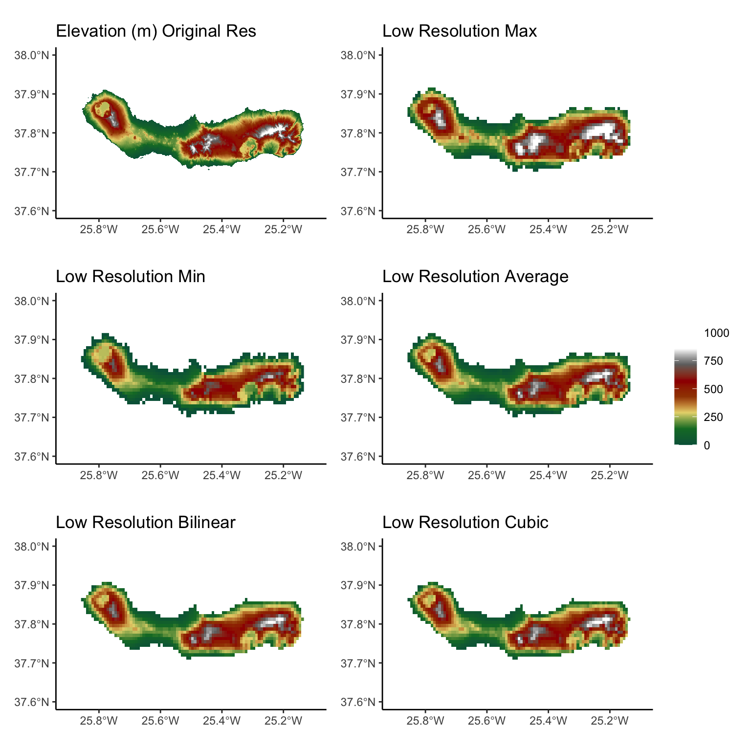
So our temperature raster is the lowest resolution (same as Precipitation) so we want to use the resample function. But we need to decide how to combine multiple values into one, we might take the mean, median, max, min, quartiles, sum or mode. The default for a continuous value is bilinear interpolation, but cubic, cubic spline, lanczos window among others are available in terra. We should chose a method that works best for our objective. For the elevation we can see what the differences will be for multiple different methods. We will set the scales to all be the same to highlight differences.

Elevation_Low_max<-resample(Elevation_SM,avgtemp_SM,method="max")
Elevation_Low_min<-resample(Elevation_SM,avgtemp_SM,method="min")
Elevation_Low_average<-resample(Elevation_SM,avgtemp_SM,method="average")
Elevation_Low_bilinear<-resample(Elevation_SM,avgtemp_SM,method="bilinear")
Elevation_Low_cubic<-resample(Elevation_SM,avgtemp_SM,method="cubic")

p5<-ggplot()+
  geom_spatraster(data=Elevation_SM)+
  labs(title="Elevation (m) Original Res",fill="")+
  scale_fill_hypso_c("dem_poster",na.value = NA,
                     limits=c(0,1000))+
  theme_classic()

p6<-ggplot()+
  geom_spatraster(data=Elevation_Low_max)+
  labs(title="Low Resolution Max",fill="")+
  scale_fill_hypso_c("dem_poster",na.value = NA,
                     limits=c(0,1000))+
  theme_classic()

p7<-ggplot()+
  geom_spatraster(data=Elevation_Low_min)+
  labs(title="Low Resolution Min",fill="")+
  scale_fill_hypso_c("dem_poster",na.value = NA,
                     limits=c(0,1000))+
  theme_classic()

p8<-ggplot()+
  geom_spatraster(data=Elevation_Low_average)+
  labs(title="Low Resolution Average",fill="")+
  scale_fill_hypso_c("dem_poster",na.value = NA,
                     limits=c(0,1000))+
  theme_classic()

p9<-ggplot()+
  geom_spatraster(data=Elevation_Low_bilinear)+
  labs(title="Low Resolution Bilinear",fill="")+
  scale_fill_hypso_c("dem_poster",na.value = NA,
                     limits=c(0,1000))+
  theme_classic()

p10<-ggplot()+
  geom_spatraster(data=Elevation_Low_cubic)+
  labs(title="Low Resolution Cubic",fill="")+
  scale_fill_hypso_c("dem_poster",na.value = NA,
                     limits=c(0,1000))+
  theme_classic()


(p5+p6)/(p7+p8)/(p9+p10)+plot_layout(guides="collect")

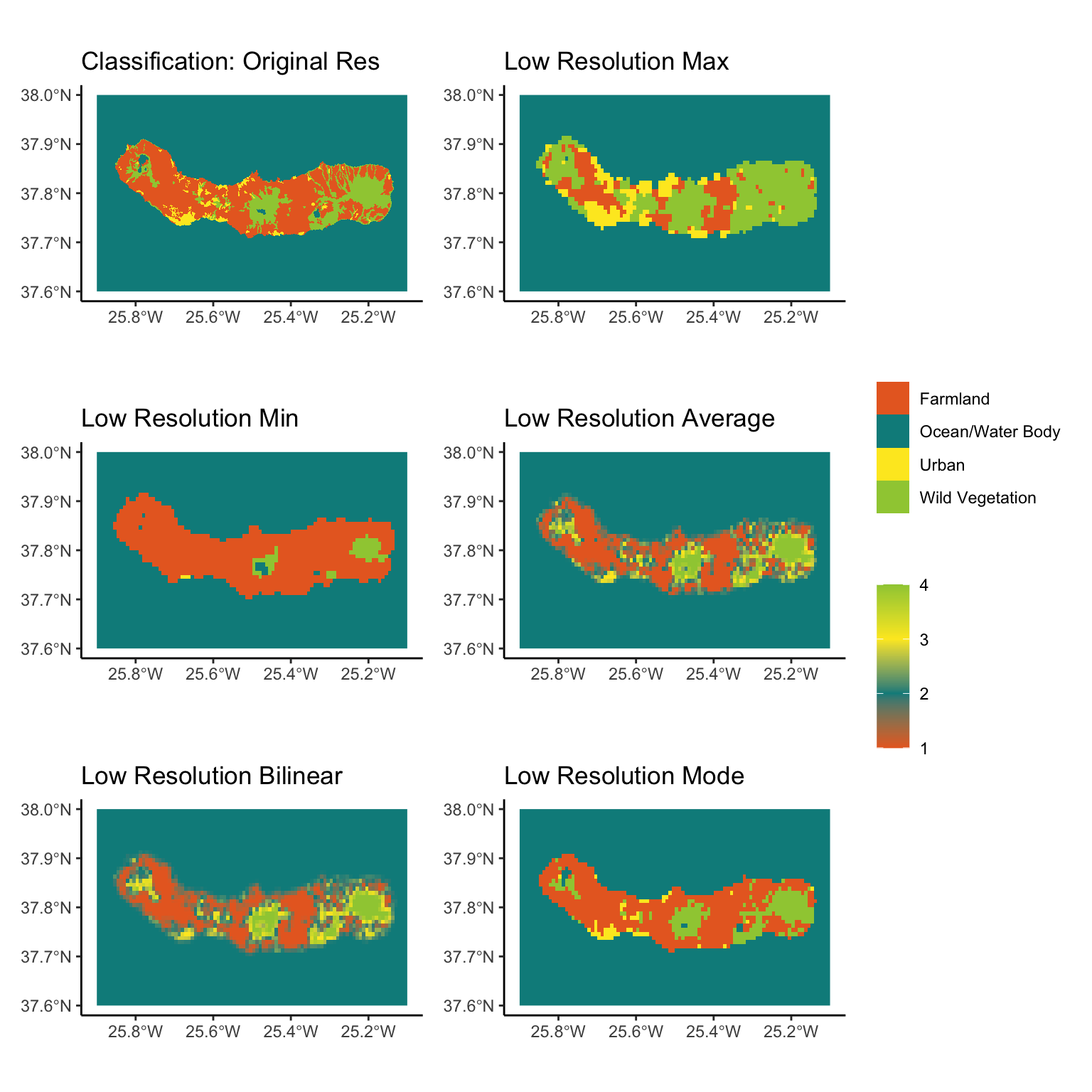
Okay this seems pretty similar but the biggest difference come from min, max and average, while bilinear, cubic and average all appear very similar. For this reason we will use bilinear for the elevation. However, for the classification we have a numeric value, but it is categorical. Therefore we will use the mode value. But lets have a look at how the others act too just to be curious.

Grouped_Classification_Low_max<-resample(Grouped_Classification,
                                         avgtemp_SM,method="max")
Grouped_Classification_Low_min<-resample(Grouped_Classification,
                                         avgtemp_SM,method="min")
Grouped_Classification_Low_average<-resample(Grouped_Classification,
                                             avgtemp_SM,method="average")
Grouped_Classification_Low_bilinear<-resample(Grouped_Classification,
                                              avgtemp_SM,method="bilinear")
Grouped_Classification_Low_mode<-resample(Grouped_Classification,
                                          avgtemp_SM,method="mode")

p11<-ggplot()+
  geom_spatraster(data=Grouped_Classification,
                  maxcell = 5e+7)+
  labs(title="Classification: Original Res",fill="")+
  scale_fill_manual(name="",
                    values = c("#e86a28",
                               "#008B8B", 
                               "#fde825", 
                               "#9fcb41"))+
  theme_classic()

p12<-ggplot()+
  geom_spatraster(data=Grouped_Classification_Low_max)+
  labs(title="Low Resolution Max",fill="")+
  scale_fill_gradientn(name="",
                       colors = c("#e86a28",
                                  "#008B8B", 
                                  "#fde825", 
                                  "#9fcb41"))+
  theme_classic()

p13<-ggplot()+
  geom_spatraster(data=Grouped_Classification_Low_min)+
  labs(title="Low Resolution Min",fill="")+
  scale_fill_gradientn(name="",
                       colors = c("#e86a28",
                                  "#008B8B", 
                                  "#fde825", 
                                  "#9fcb41"))+
  theme_classic()


p14<-ggplot()+
  geom_spatraster(data=Grouped_Classification_Low_average)+
  labs(title="Low Resolution Average",fill="")+
  scale_fill_gradientn(name="",
                       colors = c("#e86a28",
                                  "#008B8B", 
                                  "#fde825", 
                                  "#9fcb41"))+
  theme_classic()


p15<-ggplot()+
  geom_spatraster(data=Grouped_Classification_Low_bilinear)+
  labs(title="Low Resolution Bilinear",fill="")+
  scale_fill_gradientn(name="",
                       colors = c("#e86a28",
                                  "#008B8B", 
                                  "#fde825", 
                                  "#9fcb41"))+
  theme_classic()


p16<-ggplot()+
  geom_spatraster(data=Grouped_Classification_Low_mode)+
  labs(title="Low Resolution Mode",fill="")+
  scale_fill_gradientn(name="",
                       colors = c("#e86a28",
                                  "#008B8B", 
                                  "#fde825", 
                                  "#9fcb41"))+
  theme_classic()



(p11+p12)/(p13+p14)/(p15+p16)+plot_layout(guides="collect")

To make sure all extents and resolutions are the same we will resample the other rasters with the same base level/raster: temperature. This shouldn’t change anything, just sorts any odd extents or dimensions, especially small unrounded values. The method of resample won’t matter so we will leave bilinear as default. We also want to change the classification back to be a category not a number.

avgprec_Low<-resample(avgprec_SM,avgtemp_SM)
pop_density_Low<-resample(pop_density,avgtemp_SM)

Grouped_Classification_Low_mode<-Grouped_Classification_Low_mode%>% 
  tidyterra::mutate(LABEL3=case_when(LABEL3==1~"Farmland",
                                     LABEL3==2~"Ocean/Water Body",
                                     LABEL3==3~"Urban",
                                     LABEL3==4~"Wild Vegetation"))

Aggregate to Highest Resolution

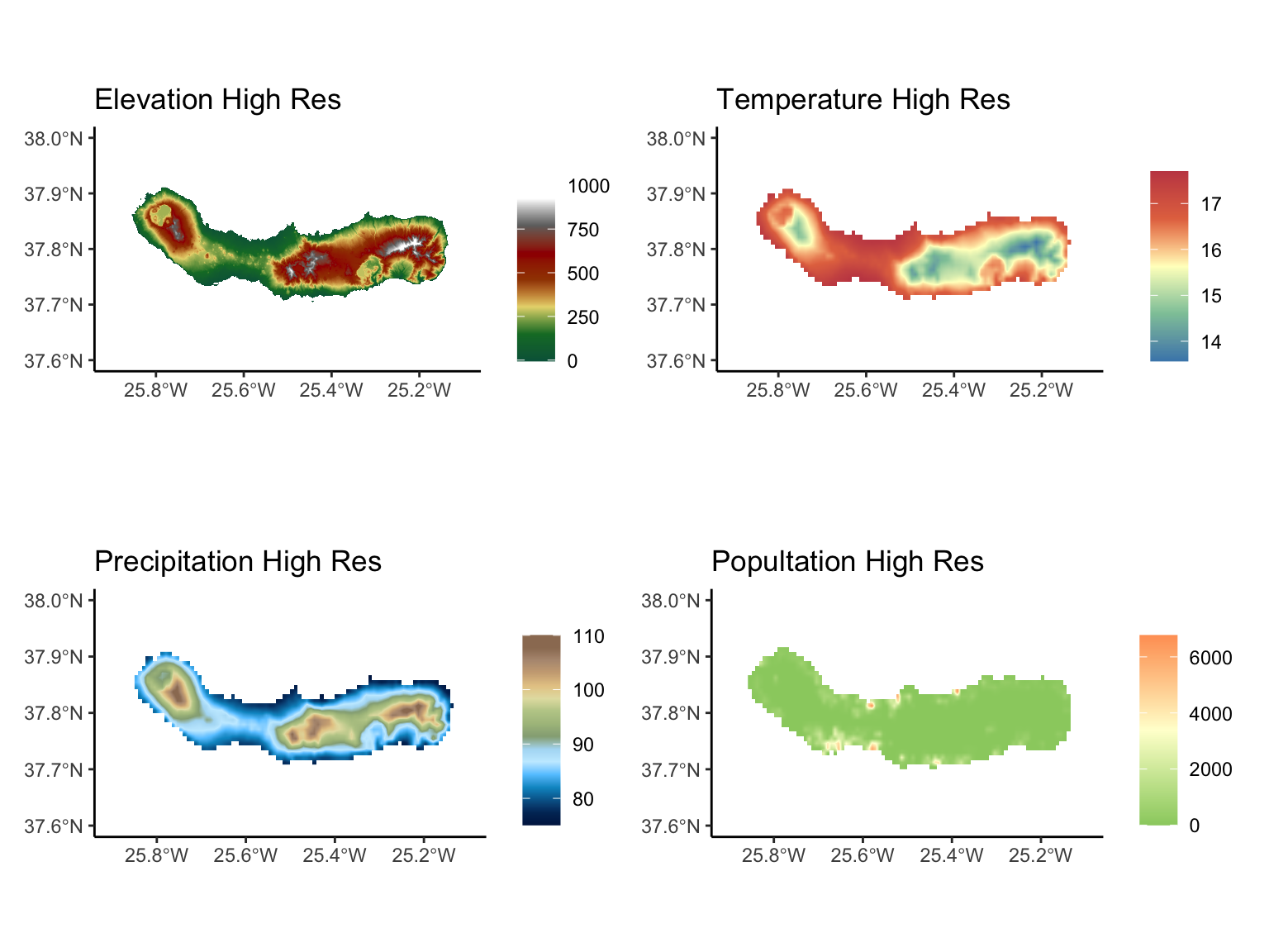
Conversely we can increase the resolution of all rasters to be the highest level. Our Classification raster is the highest so we want to use the resample function as above but this time it repeats values at higher resolution rather than combining them into one low resolution value. Again, this means the default method is fine, as all methods should return the same result.

Elevation_High<-resample(Elevation_SM,Grouped_Classification)
Temperature_High<-resample(avgtemp_SM,Grouped_Classification)
Precipitation_High<-resample(avgprec_SM,Grouped_Classification)
Population_High<-resample(pop_density,Grouped_Classification)


p17<-ggplot()+
  geom_spatraster(data=Elevation_High,
                   maxcell = 5e+7)+
  labs(title="Elevation High Res",fill="")+
  scale_fill_hypso_c("dem_poster",na.value = NA)+
  theme_classic()

p18<-ggplot()+
  geom_spatraster(data=Temperature_High,
                  maxcell = 5e+7)+
  labs(title="Temperature High Res",fill="")+
  scale_fill_whitebox_c("muted",na.value = NA)+
  theme_classic()

p19<-ggplot()+
  geom_spatraster(data=Precipitation_High,
                  maxcell = 5e+7)+
  labs(title="Precipitation High Res",fill="")+
  scale_fill_hypso_c("colombia",na.value = NA)+
  theme_classic()


p20<-ggplot()+
  geom_spatraster(data=Population_High,
                  maxcell = 5e+7)+
  labs(title="Popultation High Res",fill="")+
  scale_fill_whitebox_c("soft",na.value = NA)+
  theme_classic()



(p17+p18)/(p19+p20)

This doesn’t really change the appearance of our plots but we can see the resolution is now higher.

Combining

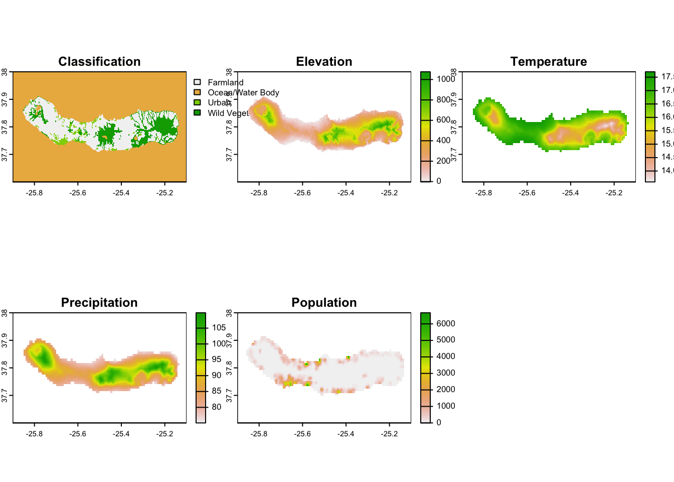
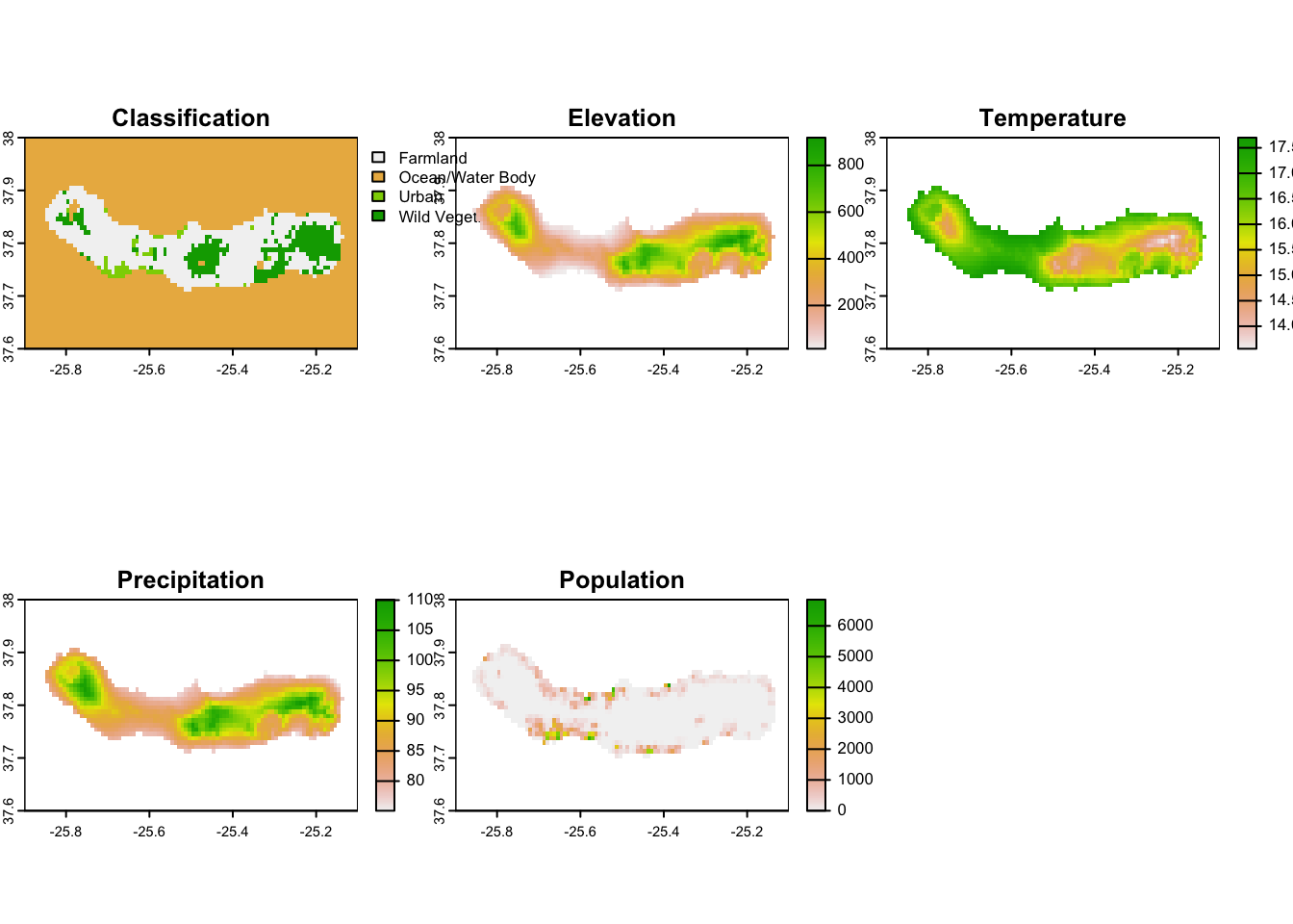
We can just use the c() function to add layers of a raster together into one multi layer or band raster. When we have a multilayer raster like this but the bands have different scales, plotting them with ggplot and tidyterra doesn’t really work easily, but thankfully the base plot function works reasonably well just for quick inspection.

Combined_HighRes<-c(Grouped_Classification,
                    Elevation_High,
                    Temperature_High,
                    Precipitation_High,
                    Population_High)

names(Combined_HighRes)<-c("Classification",
                           "Elevation",
                           "Temperature",
                           "Precipitation",
                           "Population")

plot(Combined_HighRes)

Combined_LowRes<-c(Grouped_Classification_Low_mode,
                   Elevation_Low_bilinear,
                   avgtemp_SM,
                   avgprec_Low,
                   pop_density_Low)

names(Combined_LowRes)<-c("Classification",
                          "Elevation",
                          "Temperature",
                          "Precipitation",
                          "Population")

plot(Combined_LowRes)

Analysing

Visual Inspection

For many of the analysis methods, formal and informal, we will probably want our data to be in a tibble format. Then we can look at how to compare the different classes. Firstly, most of our environmental data is terrestrial so we can remove all the ocean areas. Then compare environmental data across classes and if the different spatial resolutions change this relationship.

LowRes_df<-as.data.frame(Combined_LowRes,xy=T) %>% 
  mutate(Res="Low")

HighRes_df<-as.data.frame(Combined_HighRes,xy=T)%>% 
  mutate(Res="High")

HighRes_df %>% 
  bind_rows(LowRes_df) %>% 
  drop_na() %>% 
  pivot_longer(-c(x,y,Classification,Res),
               names_to = "Metric",values_to = "value")%>% 
  ggplot(aes(x=Classification,y=value,fill=Res))+
  geom_boxplot()+
  facet_wrap(~Metric,scales = "free")+
  scale_fill_manual(name="Resolution",
                    values=c("#36b779","#2d85c5"))+
  theme_classic()

Incorrect Formal Analysis (Just an Example)

Generally the same patterns are in high and low (not surprisingly). To give a little example analysis we could create a model based on the low resolution environmental data, and see if we can accurately predict the high resolution classification. This won’t be the best or most effective way at doing this task, but an example! DO NOT EMULATE THIS EXCEPT AS A LEARNING EXERCISE (Check other tutorials for applying models correctly, what steps to take and best practices). For example, if you look at temperature, elevation, precipitation for example they are clearly correlated so would require more complex modelling to do correctly.

lowres_Model<-nnet::multinom(Classification~Elevation+
                         Temperature+
                         Precipitation+
                         Population,
                       data=LowRes_df)

# weights:  24 (15 variable)
initial  value 1497.197910 
iter  10 value 888.197723
iter  20 value 657.680242
iter  30 value 644.902880
iter  40 value 644.384735
iter  40 value 644.384732
final  value 644.383545 
converged

HighRes_df$Pred<-predict(lowres_Model,
                         newdata=HighRes_df,"class")

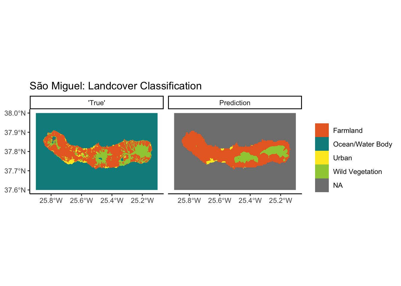
So now we have a prediction and a “true” class at high resolution, lets convert back to raster and compare the true and predicted maps. To do this we convert our dataframe to an sf object, create an empty rast() with the same resolution, crs and extent as our original high resolution rast, then fill the empty raster with our predictions from the model, we use a min function but actually it should not summarise at all. Then we can stack the true and the predicted rasters together to visualise the difference.

HighRes_sf<-st_as_sf(HighRes_df,coords=c("x","y"))


HighRes_Pred_raster <- rast(resolution = res(Grouped_Classification),
                               crs = crs(Grouped_Classification),
                               ext = ext(Grouped_Classification)) %>% 
  rasterize(vect(HighRes_sf), ., field = "Pred", fun = "min")%>% 
  tidyterra::mutate(Pred_min=case_when(
    Pred_min==0~"Farmland",
    Pred_min==1~"Ocean/Water Body",
    Pred_min==2~"Urban",
    Pred_min==3~"Wild Vegetation"))


HighRes_True_Pred_raster<-c(Grouped_Classification,
                            HighRes_Pred_raster)

names(HighRes_True_Pred_raster)<-c("'True'","Prediction")

ggplot()+
  geom_spatraster(data=HighRes_True_Pred_raster,
                  maxcell = 5e+7
                  )+
  labs(title="São Miguel: Landcover Classification")+
  facet_wrap(~lyr)+
  scale_fill_manual(name="",
                    values = c("#e86a28",
                               "#008B8B", 
                               "#fde825", 
                               "#9fcb41"))+
  theme_classic()

Actually not a very good prediction, but that is not surprising given the model that was used and the little input data used. We will go through some remote sensing tutorials and then we can apply Machine Learning methods alongside spatial data skills to create some prediction models that will hopefully do a lot better.